Vanishing Gradient Problem
Why gradients can shrink across many layers or timesteps, and why long-range learning becomes difficult.
Background
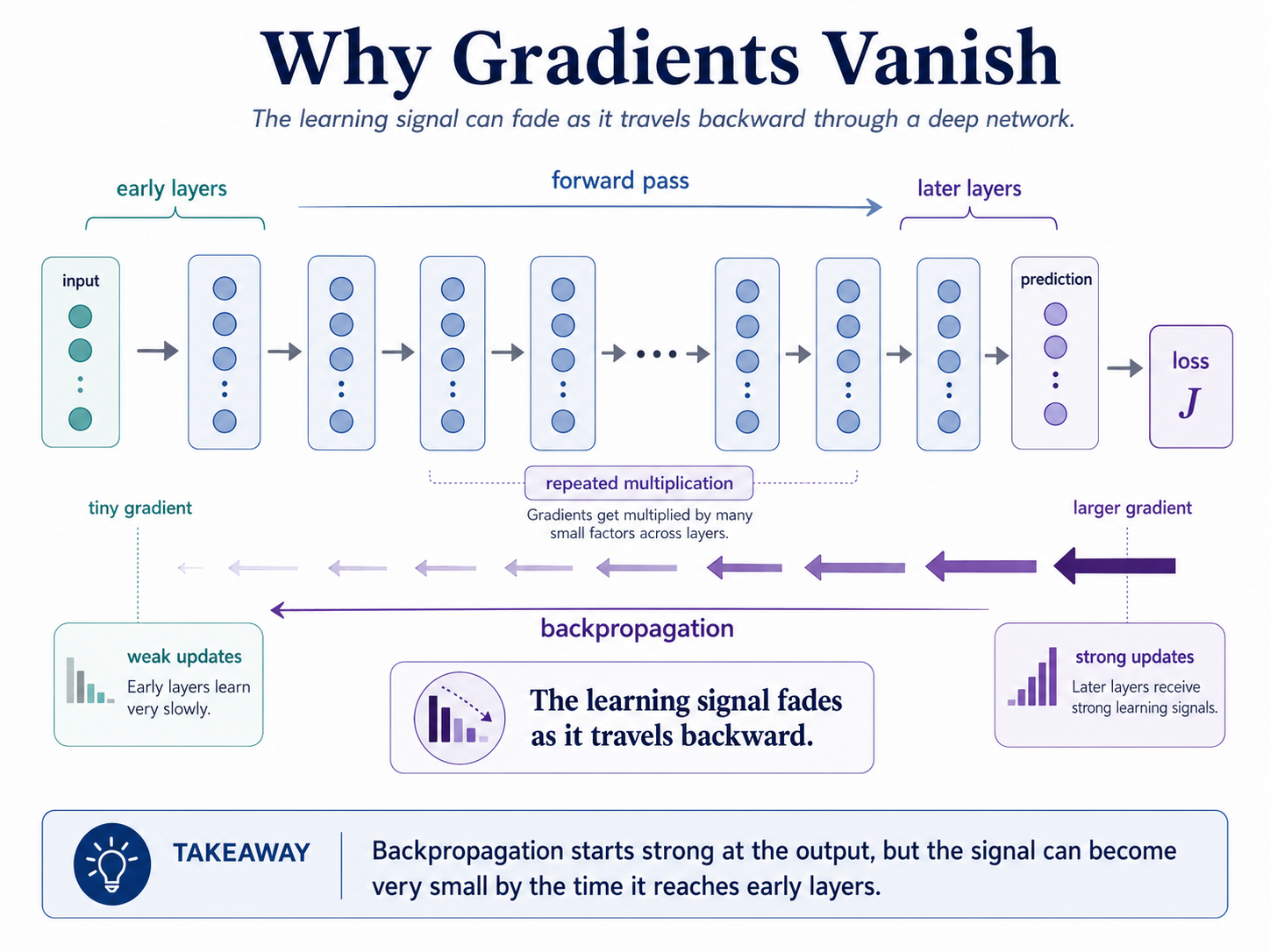
Deep networks are powerful because they stack many layers. Each layer transforms the input a little more, helping the model build richer representations.
But learning does not only move forward. During training, the model also sends gradients backward from the loss to earlier layers. These gradients are the learning signals that tell each weight how to change.
In a very deep network, the backward signal must pass through many layers. If each layer shrinks it a little, the signal can become extremely small by the time it reaches the early layers.
That means later layers may keep learning, while early layers receive tiny updates and barely change. This is the vanishing gradient problem.
Idea
The core idea is: the learning signal fades as it travels backward.
During backpropagation, gradients are passed backward using the chain rule. Each step multiplies the gradient by a local derivative.
If many of those derivatives are smaller than 1, the gradient keeps shrinking: small x small x small x small becomes very small.
The problem is not that the model has no gradient anywhere. The problem is that the gradient becomes too small by the time it reaches earlier layers.
Sigmoid and tanh saturation can make this worse, because their derivatives can become very small. This does not mean sigmoid is always bad; the issue is that many small derivatives multiplied together can shrink the backward signal.
Formula
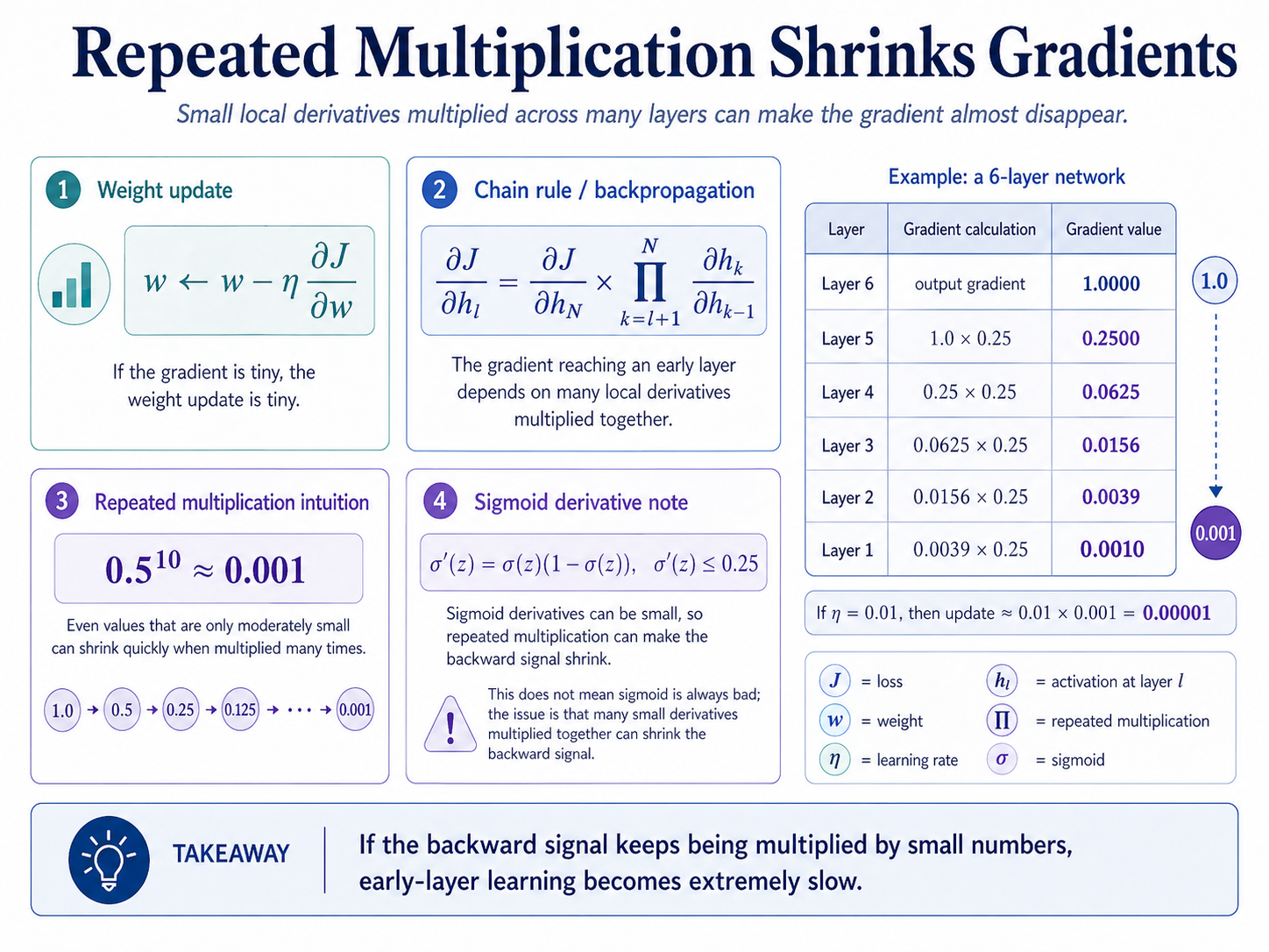
Gradient descent updates a weight using the gradient of the loss.
Backpropagation sends gradients backward through repeated multiplication.
Even a moderately small factor can shrink quickly when multiplied many times.
Sigmoid derivatives are at most 0.25, so repeated sigmoid-like derivatives can shrink gradients.
Symbols
- J: loss function.
- w: model weight.
- eta: learning rate.
- partial J / partial w: gradient of the loss with respect to a weight.
- h_l: activation or representation at layer l.
- h_N: activation or representation at final layer N.
- partial h_k / partial h_{k-1}: local derivative from one layer to the previous layer.
- prod: product or repeated multiplication.
- sigma(z): sigmoid activation.
- sigma'(z): derivative of sigmoid.
- N: final layer index.
Example
Imagine a 6-layer network. The output layer starts with a gradient of 1.0.
As the gradient moves backward, each layer multiplies it by a local derivative of 0.25.
Layer 6 starts at 1.0000. Layer 5 receives 1.0 x 0.25 = 0.2500. Layer 4 receives 0.2500 x 0.25 = 0.0625. Layer 3 receives 0.0156. Layer 2 receives 0.0039. Layer 1 receives about 0.0010.
By the time the gradient reaches Layer 1, it is close to zero.
If the learning rate is eta = 0.01, then the update is 0.01 x 0.001 = 0.00001. That is a very small change.
The early layer is technically learning, but it is learning so slowly that progress can feel almost frozen.
Workflow
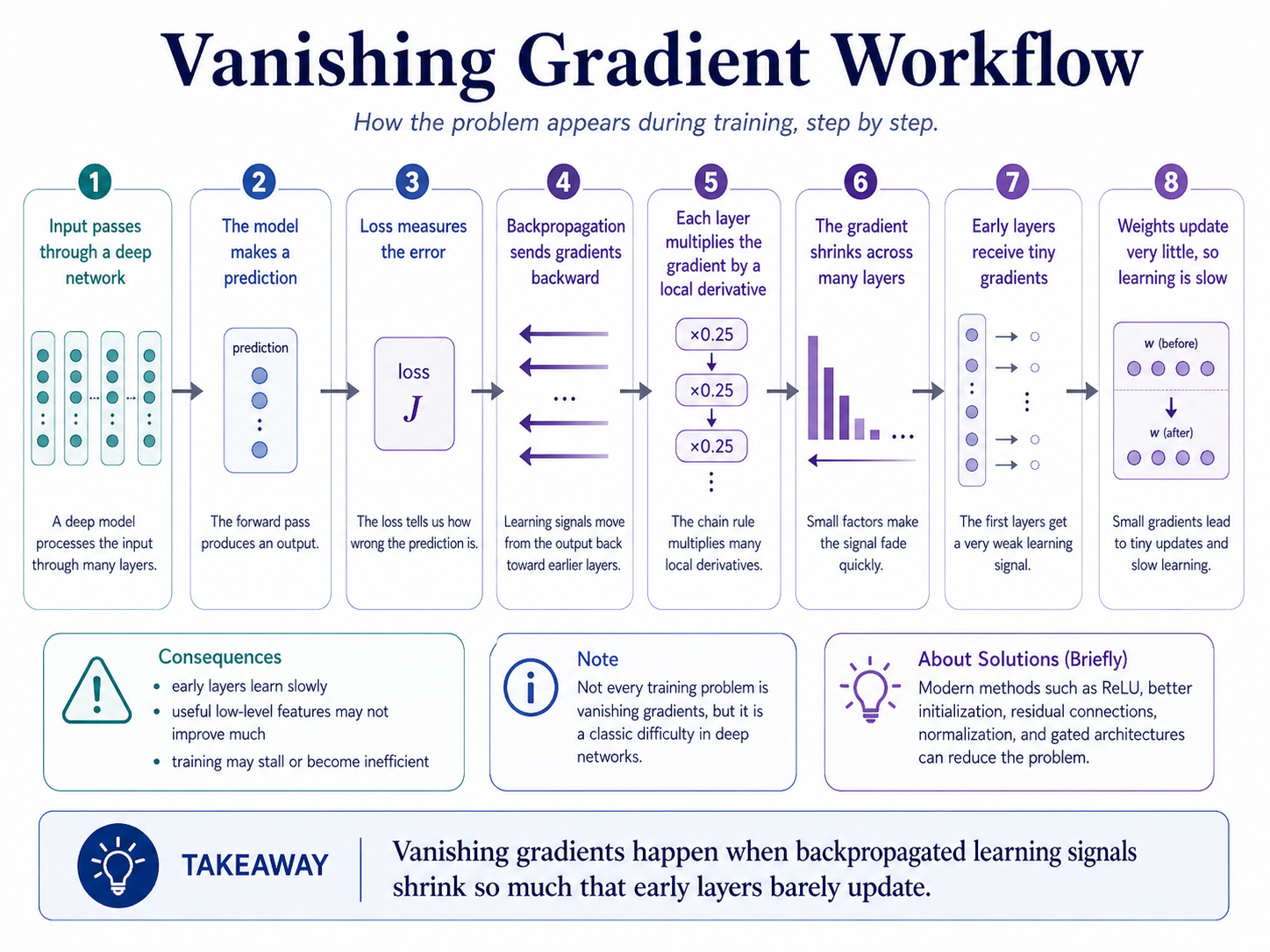
- A deep network makes a prediction.
- The loss measures how wrong the prediction is.
- Backpropagation sends gradients from the output layer backward.
- Each layer multiplies the gradient by its local derivative.
- If many local derivatives are smaller than 1, the gradient shrinks.
- Early layers receive very small gradients.
- Their weights update very little.
- The network learns slowly or fails to learn useful early features.
Why Understanding It Helps
- Explains why very deep networks can be hard to train.
- Helps beginners understand why activation choice matters.
- Explains why good initialization is important.
- Shows why residual connections and skip connections help gradients flow.
- Helps diagnose why early layers may learn slowly.
Limitations of This Explanation
- Not every training failure is caused by vanishing gradients.
- Small gradients can also come from poor learning rates, bad initialization, or saturated activations.
- The opposite problem, exploding gradients, can also happen.
- ReLU-like activations, normalization, residual connections, and gated architectures can reduce the problem, but they do not make training automatically easy.
- This explanation focuses on the problem, not the full set of modern solutions.
Takeaway
The vanishing gradient problem happens when the learning signal becomes smaller as it travels backward through many layers.
When early layers receive tiny gradients, their weights barely update.
If the backward signal keeps being multiplied by small numbers, learning fades.