Optimization

RMSProp

Learn how RMSProp gives each parameter an adaptive step size by tracking recent squared gradients.

Background

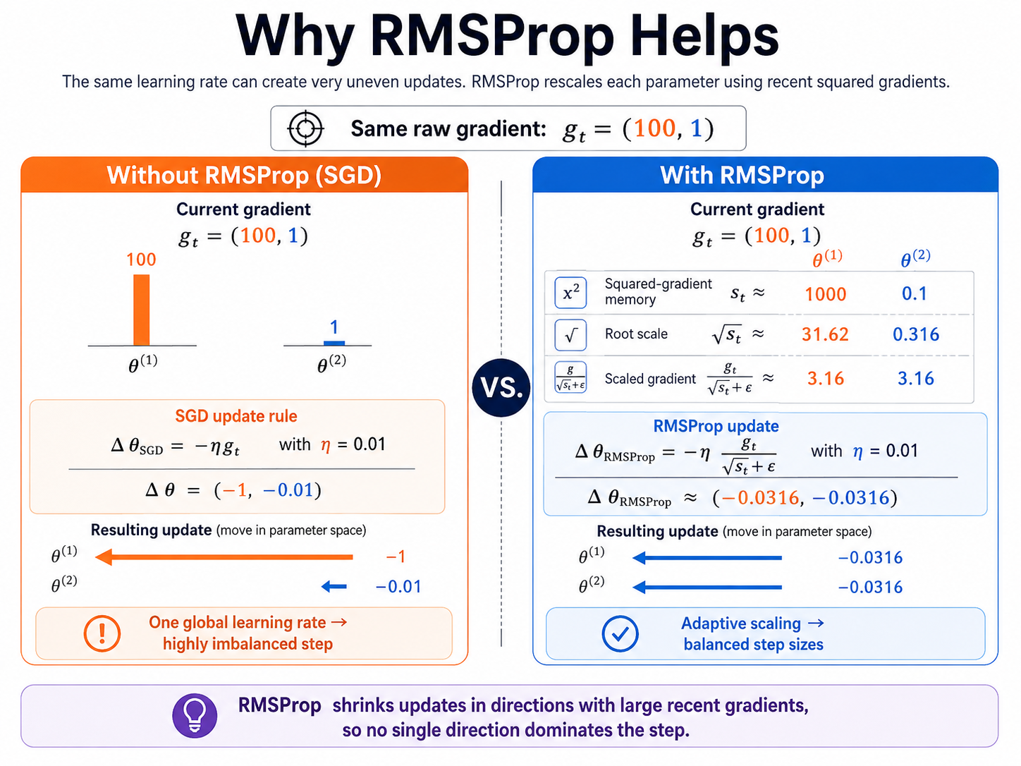
Plain SGD uses one global learning rate for every parameter. This is simple, but it can be hard to tune when different parameters have very different gradient scales.

If one direction has very large gradients, SGD may take unstable steps in that direction. If another direction has small gradients, SGD may move too slowly there.

RMSProp solves this by tracking recent squared gradients. Instead of using the raw gradient directly, it divides each gradient component by a running root-mean-square scale.

RMSProp is different from Momentum. Momentum remembers direction. RMSProp remembers scale.

Idea

The core idea is: large recent gradients create a larger denominator, which creates a smaller effective step.

SGD uses one learning rate. RMSProp creates a different effective learning rate for each parameter by looking at the recent squared-gradient magnitude.

This makes RMSProp helpful on badly scaled surfaces, where one parameter direction can otherwise dominate the update.

Important Formulas

\[g_t=\frac{1}{B}\sum_{i\in\mathcal{B}_t}\nabla_\theta \ell_i(\theta_t)\]

Mini-batch gradient input. RMSProp starts with the same gradient as SGD.

\[\theta_{t+1}=\theta_t-\eta g_t\]

Plain SGD applies the same learning rate to every parameter.

\[s_t=\rho s_{t-1}+(1-\rho)(g_t\odot g_t)\]

Squared-gradient accumulator. It stores recent gradient magnitude, not direction.

\[\theta_{t+1}=\theta_t-\eta\frac{g_t}{\sqrt{s_t}+\epsilon}\]

RMSProp scales the gradient element-wise before updating the parameters.

\[\eta_{\text{eff},j}=\frac{\eta}{\sqrt{s_{t,j}}+\epsilon}\]

Effective learning rate for one parameter j.

\[s_t=(1-\rho)(g_t\odot g_t)+(1-\rho)\rho(g_{t-1}\odot g_{t-1})+(1-\rho)\rho^2(g_{t-2}\odot g_{t-2})+\cdots\]

Expanded memory view: recent squared gradients matter more, while older ones fade.

\[s_{dW,t}^{[l]}=\rho s_{dW,t-1}^{[l]}+(1-\rho)(dW_t^{[l]}\odot dW_t^{[l]})\]

Layer-wise RMSProp accumulator for weight gradients.

\[s_{db,t}^{[l]}=\rho s_{db,t-1}^{[l]}+(1-\rho)(db_t^{[l]}\odot db_t^{[l]})\]

Layer-wise RMSProp accumulator for bias gradients.

\[W_{t+1}^{[l]}=W_t^{[l]}-\eta\frac{dW_t^{[l]}}{\sqrt{s_{dW,t}^{[l]}}+\epsilon}\]

Layer-wise weight update.

\[b_{t+1}^{[l]}=b_t^{[l]}-\eta\frac{db_t^{[l]}}{\sqrt{s_{db,t}^{[l]}}+\epsilon}\]

Layer-wise bias update.

Symbols

g_t: mini-batch gradient at step t.
eta: global learning rate.
s_t: running average of recent squared gradients.
rho: decay rate for the accumulator.
epsilon: small value for numerical stability.
odot: element-wise multiplication.
eta_eff,j: effective learning rate for parameter j.

Pros

Pros	Why it helps
Adaptive per-parameter scaling	RMSProp adjusts each update based on recent gradient magnitude.
Helpful on badly scaled surfaces	It reduces unstable movement in directions with consistently large gradients.
Less dependent on one perfect learning rate	The global learning rate still matters, but each parameter gets its own effective step size.
Important bridge to Adam	Adam uses a similar squared-gradient accumulator as part of its adaptive scaling.
Works with noisy mini-batches	Recent squared-gradient memory smooths sudden gradient-scale changes.

Cons

Cons	Why it matters
Adds hyperparameters	Rho, eta, and epsilon must be chosen sensibly.
Can shrink useful directions too much	Large accumulated squared gradients can make a parameter's effective step very small.
No direction memory	RMSProp rescales gradients, but Momentum is still the idea that smooths direction.
Less transparent than SGD	The effective learning rate changes per parameter over time.
Often replaced by Adam	Adam combines Momentum-like direction memory with RMSProp-like scaling.

Quick Example

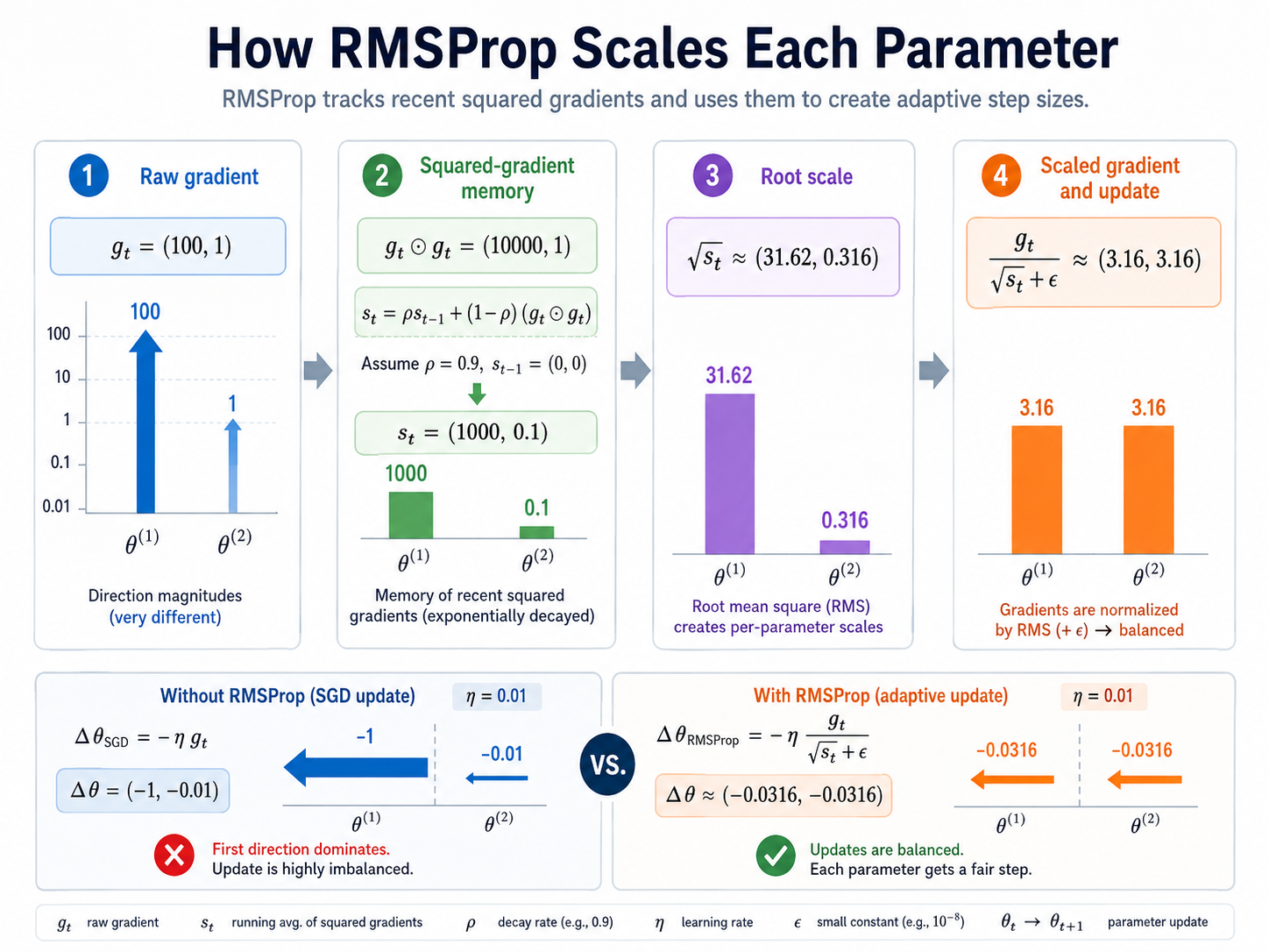
Suppose two parameters have the same global learning rate but very different gradient magnitudes. Let theta_t = (0, 0), g_t = (100, 1), and eta = 0.01.

Plain SGD would update by eta g_t = (1, 0.01), so the first parameter dominates the movement.

With RMSProp, use rho = 0.9, s_{t-1} = (0, 0), and ignore epsilon only for this simplified calculation. The squared-gradient accumulator becomes s_t = (1000, 0.1), so the root scale is approximately (31.62, 0.316).

RMSProp scales raw gradients into balanced parameter updates — Image 2: RMSProp turns uneven raw gradients into more balanced updates.

Example Calculation

\[\eta g_t=0.01(100,1)=(1,0.01)\]

Plain SGD produces a highly imbalanced update.

\[s_t=0.9(0,0)+0.1(10000,1)=(1000,0.1)\]

RMSProp stores recent squared-gradient magnitude.

\[\sqrt{s_t}\approx(31.62,0.316)\]

The larger-gradient direction receives a larger denominator.

\[\frac{g_t}{\sqrt{s_t}+\epsilon}\approx\frac{(100,1)}{(31.62,0.316)}\approx(3.16,3.16)\]

The scaled gradient becomes balanced.

\[\theta_{t+1}\approx(0,0)-0.01(3.16,3.16)=(-0.0316,-0.0316)\]

The large-gradient direction no longer dominates the step.

Common Mistakes

Thinking RMSProp changes how g_t is computed. It does not; it changes how the gradient is scaled before the update.
Confusing RMSProp with Momentum. Momentum remembers past gradient directions; RMSProp remembers past squared-gradient magnitudes.
Forgetting that the square, square root, and division are element-wise operations.
Thinking RMSProp removes the need for learning-rate tuning. The global learning rate eta still matters.
Confusing RMSProp with Adam. Adam tracks both a first moment and a second moment, then applies bias correction.

Takeaway

RMSProp gives each parameter an adaptive step size by tracking recent squared gradients.

Directions with consistently large gradients receive smaller effective steps, while directions with smaller gradients are not suppressed as much.

Momentum remembers direction. RMSProp remembers scale. Adam later combines both ideas.