Optimization

Momentum

Learn how Momentum gives gradient descent memory, reducing zig-zag movement and building speed in consistent directions.

Background

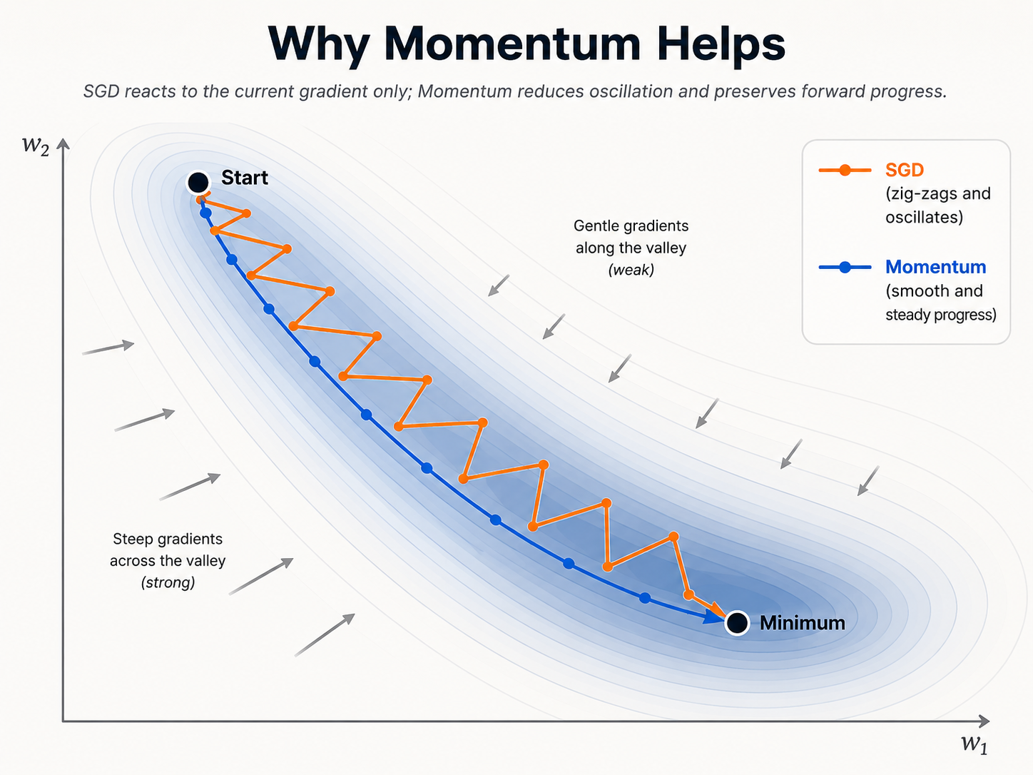
Plain SGD updates parameters using only the current gradient. This is simple, but it can be unstable when the loss surface has a narrow valley.

In a narrow valley, the gradient may be steep across the valley but weak along the valley. As a result, SGD can bounce from side to side instead of moving smoothly forward.

Momentum adds memory to the optimizer. Instead of trusting only the current gradient, it combines the current gradient with a running average of past gradients.

Momentum strengthens directions that stay consistent and weakens directions that keep flipping. This helps the optimizer move more smoothly through ravines and curved valleys.

Idea

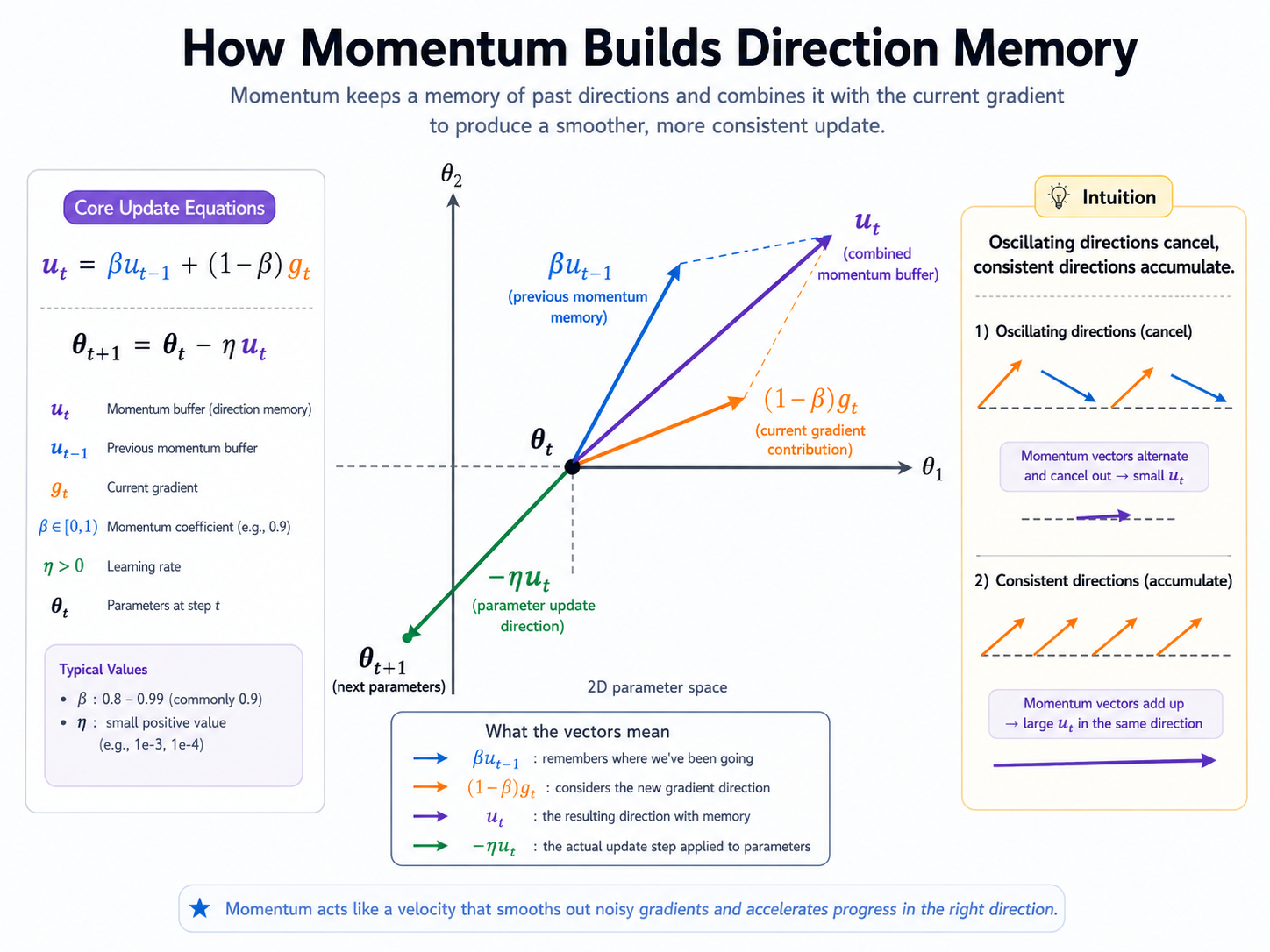
The core idea is: current gradient plus past direction memory gives a smoother update direction.

If gradients keep pointing in a similar direction, the momentum buffer builds in that direction. If gradients keep flipping direction, the buffer weakens that oscillating direction.

Momentum is therefore not only about speed. It changes the optimization path by making consistent movement stronger and unstable movement weaker.

Momentum buffer combines previous momentum and current gradient — Image 2: The momentum buffer stores direction memory before the parameter update.

Important Formulas

\[g_t=\frac{1}{B}\sum_{i\in\mathcal{B}_t}\nabla_\theta \ell_i(\theta_t)\]

Mini-batch gradient input. Momentum changes how gradients are remembered, not how this gradient is computed.

\[\theta_{t+1}=\theta_t-\eta g_t\]

Plain SGD reacts directly to the current mini-batch gradient.

\[u_t=\beta u_{t-1}+(1-\beta)g_t\]

Momentum buffer: a smoothed gradient direction with memory.

\[\theta_{t+1}=\theta_t-\eta u_t\]

The parameter update uses the momentum buffer instead of the raw gradient.

\[u_t=(1-\beta)g_t+(1-\beta)\beta g_{t-1}+(1-\beta)\beta^2 g_{t-2}+(1-\beta)\beta^3 g_{t-3}+\cdots\]

Expanded memory view: recent gradients matter more, while older gradients fade gradually.

\[u_{dW,t}^{[l]}=\beta u_{dW,t-1}^{[l]}+(1-\beta)dW_t^{[l]}\]

Layer-wise momentum buffer for weight gradients.

\[u_{db,t}^{[l]}=\beta u_{db,t-1}^{[l]}+(1-\beta)db_t^{[l]}\]

Layer-wise momentum buffer for bias gradients.

\[W_{t+1}^{[l]}=W_t^{[l]}-\eta u_{dW,t}^{[l]}\]

Layer-wise weight update.

\[b_{t+1}^{[l]}=b_t^{[l]}-\eta u_{db,t}^{[l]}\]

Layer-wise bias update.

Symbols

g_t: mini-batch gradient at step t.
B: mini-batch size.
theta_t: model parameters before the update.
eta: learning rate.
u_t: momentum buffer, or smoothed gradient direction.
beta: momentum coefficient, often around 0.9.
dW_t and db_t: weight and bias gradients for one layer.

Pros

Pros	Why it helps
Reduces zig-zag movement	Momentum smooths directions that change too quickly across steps.
Speeds up consistent progress	When gradients keep pointing in a useful direction, the buffer builds movement in that direction.
Smooths mini-batch noise	One noisy mini-batch has less control over the update direction.
Simple and memory-efficient	It only adds one extra buffer for each parameter.
Strong practical baseline	SGD with Momentum is still powerful when the learning rate is tuned well.

Cons

Cons	Why it matters
Adds one more hyperparameter	The momentum coefficient beta must be chosen carefully.
Can overshoot	If the learning rate or momentum is too large, the optimizer may move past a good region.
No per-parameter scaling	Momentum smooths direction, but does not automatically resize each parameter step like RMSProp or Adam.
Still needs learning-rate tuning	Momentum helps the path, but a bad learning rate can still make training unstable.
Notation varies	Different books may write Momentum with different signs or scaling conventions.

Quick Example

Suppose the optimizer is moving through a narrow valley. Let beta = 0.9, and assume the first two gradients are g_1 = (10, 1) and g_2 = (-9, 1).

The first coordinate changes direction sharply, but the second coordinate stays positive. Start with u_0 = (0, 0).

Example Calculation

\[u_1=0.9(0,0)+0.1(10,1)=(1,0.1)\]

The first update stores a small version of the first gradient.

\[u_2=0.9(1,0.1)+0.1(-9,1)=(0,0.19)\]

The oscillating first coordinate cancels, while the consistent second coordinate accumulates.

Common Mistakes

Thinking Momentum changes how g_t is computed. It does not; it changes how current and past gradients are combined before the update.
Confusing beta with the learning rate. Eta controls step size; beta controls how much past direction is remembered.
Using too much Momentum with too large a learning rate, which can cause overshooting or unstable movement.
Confusing Momentum's u_t with Adam's v_t. Momentum stores direction memory; Adam's v_t usually stores squared-gradient magnitude.
Thinking Momentum only makes training faster. It also changes the path by reducing oscillation.

Takeaway

SGD follows the current gradient directly. Momentum gives SGD memory by keeping a moving average of past gradients.

Directions that stay consistent become stronger, while directions that keep flipping become weaker. This makes the optimization path smoother, especially in narrow valleys where plain SGD tends to zig-zag.