Training stability

Batch Normalization

How normalization, running statistics, gamma, and beta keep deep network activations easier to train.

Without BatchNorm and with BatchNorm activation distributions — Image 1: Without BatchNorm vs. With BatchNorm activation distributions.

Background

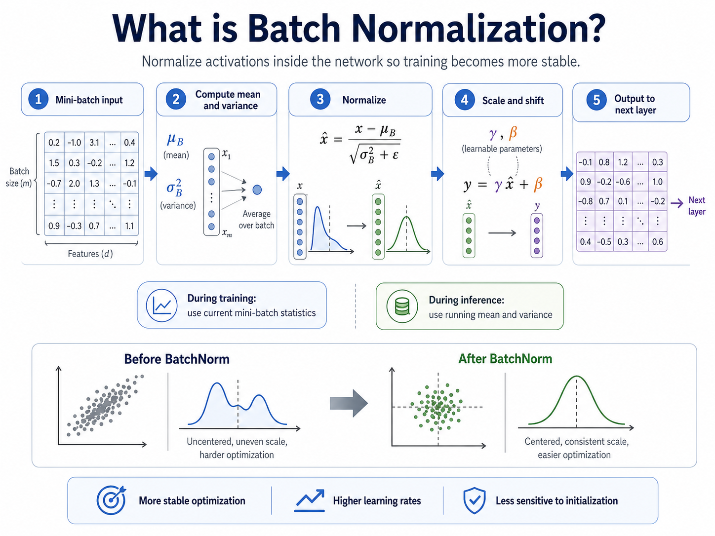
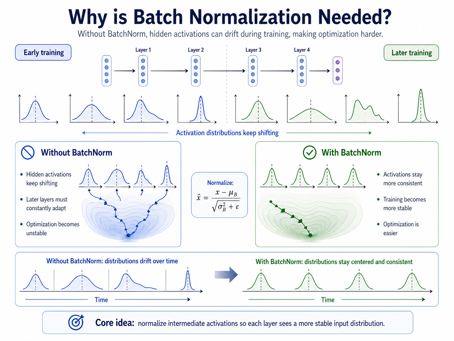
Deep networks do not only process the raw input data. Each hidden layer produces activations, and those activations become the input to the next layer.

During training, earlier layers keep changing, so later layers may receive signals whose scale and distribution keep shifting. This makes optimization harder because each layer is trying to learn from a moving target.

Batch Normalization exists to make these internal signals more stable, which can make training faster, smoother, and less fragile.

Idea

BatchNorm looks at a mini-batch of activations inside the network. It computes the mean and variance of those activations, then normalizes them so the signal becomes more centered and consistently scaled.

But BatchNorm does not simply force every signal to stay fixed forever. After normalization, it gives the model two learnable parameters: gamma for scale and beta for shift.

The mental model is simple: standardize the signal, then let the network adjust it.

Image 2: Why Batch Normalization is needed.

Formula

\[\hat{x}=\frac{x-\mu_B}{\sqrt{\sigma_B^2+\epsilon}}\]

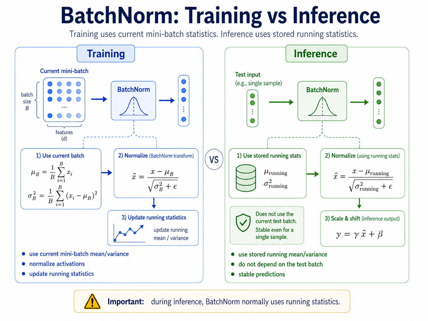
This standardizes the activation using mini-batch statistics.

\[y=\gamma\hat{x}+\beta\]

This lets the model learn the final scale and shift.

\[y=\gamma\frac{x-\mu_{\text{running}}}{\sqrt{\sigma_{\text{running}}^2+\epsilon}}+\beta\]

During inference, BatchNorm usually uses stored running statistics.

Example

Suppose one hidden feature in a mini-batch has activations x = [2, 4, 6, 8]. The mini-batch mean is mu_B = 5, and the mini-batch variance is sigma_B^2 = 5.

After normalization, x-hat is approximately [-1.34, -0.45, 0.45, 1.34]. The original activations were spread around 2, 4, 6, and 8; after normalization, they are centered around 0 and placed on a more consistent scale.

Now suppose BatchNorm has learned gamma = 2 and beta = 0.5. The final output becomes y = 2 x-hat + 0.5, approximately [-2.18, -0.40, 1.40, 3.18]. BatchNorm stabilizes the signal without removing flexibility.

BatchNorm training versus inference — Image 3: Training vs. inference.

Workflow

Input activations arrive from a hidden layer.
BatchNorm computes the mini-batch mean.
BatchNorm computes the mini-batch variance.
The activations are normalized by subtracting the mean and dividing by the standard deviation.
The model scales the normalized signal with gamma.
The model shifts the signal with beta.
The next layer receives a more stable signal.

Pros

Pros	Why it helps
More stable training	Hidden activations stay within a more controlled range.
Often allows larger learning rates	The optimizer can take bigger steps without the signal becoming too unstable.
Helps deep networks train more reliably	Later layers receive inputs that shift less dramatically during training.
Mild regularization-like effect	Mini-batch statistics vary slightly, which can add useful training noise.

Cons

Cons	Why it matters
Depends on reliable batch statistics	If the mini-batch is not representative, the normalization can be noisy.
Small batch sizes can be unstable	With too few examples, the mean and variance estimates may be poor.
Training and inference behave differently	Training uses batch statistics, while inference uses stored running statistics.
Other methods may be better sometimes	LayerNorm or GroupNorm can work better for small batches or sequence models.

Takeaway

BatchNorm is an internal signal stabilizer. It standardizes hidden activations, then learns the best scale and shift using gamma and beta.

The key idea is to make the signal easier to train on without removing the model's flexibility.